Interviews are challenging. Job interviews that require any sort of tracking data or simple calculations are even trickier, as this would require a knack of MS-Excel.
Excel usage has been increasing in the industry; individuals manage their data in Excel to analyze the business trend. And, it could be nerve-wracking for both the interviewer and the interviewee to face such questions. To prepare you for those frequently asked questions, here we present a library of 30 questions and answers picked from real interviews.
All the best!
All the best!
Q1. What is Microsoft Excel?
Answer: Microsoft Excel is an electronic spreadsheet program, created by multiple highly skilled engineers from Microsoft. It enables users to organize, format, and calculate data with formulas using a spreadsheet system broken up by rows and column.
We also use this tool for storing, organizing and manipulating the data. In addition, it also offers programming that supports VBA, and we can use external database to make dynamic reports, analysis etc. Smart use of this program saves a lot of time and helps in creating our own applications too.
Q2. What is Ribbon in MS-Excel?
Answer: The ribbon in Excel consists of the tabs at the top. These tabs are split into groups which categorize related command buttons into sub tasks.
Each group has its respective command button and the dialog box launcher, which are present in the lower right corner in some of the groups.
This opens a dialog box containing a bunch of additional options we can choose from.

As per Excel’s default settings, we have 8 tabs. Which are:
- File
- Home
- Insert
- Page Layout
- Formulas
- Data
- Review
- View
To know more in detail click here
Q3. How many rows and columns are there in Microsoft Excel 2003 and later versions?
Answer: Refer to the table below for the number of rows, columns and cells for Microsoft Excel 2003 & later version:-
| Excel Versions | Rows | Columns | Total Cells |
|---|---|---|---|
| MS Excel 2003 | 65536 | 256 | 16777216 |
| MS Excel 2007 | 1048576 | 16384 | 17179869184 |
| MS Excel 2010 | 1048576 | 16384 | 17179869184 |
| MS Excel 2013 | 1048576 | 16384 | 17179869184 |
Q4. Which option do we use to adjust the text within a cell and what is the procedure to do it?
Answer: To adjust text in a cell, we use Wrap text option. It can be used in two ways:
Option 1: In the Home tab > Alignment > Wrap Text.

Option 2:
- Press Ctrl+1 on your keyboard
- Format cells dialog box will appear
- In the Alignment Tab
- Click on Wrap text
- And then click on OK

Check for more examples:
Q5. What is the shortcut to put the filter on data in Microsoft Excel 2013?
Answer: Ctrl+Shift+L is the shortcut key to put the filter in data.
You can find more shortcuts on the below links:
250 Excel Keyboard Shortcuts
The Best Shortcut Keys
Q6. How many report formats are available in Excel and what are their names?
Answer: In Excel, we have three formats available:
- Compact
- Report
- Tabular
Q7. What is the difference between function and formula in MS-Excel?
Answer:
| Basis | Formula | Function |
|---|---|---|
| Definition | A formula is a statement written by the user to be calculated. | A function is a piece of code designed to calculate specific values and are used inside formulas. |
| Location | A formula can be typed directly into the formula bar | A function cannot be typed as its built into the software |
| Nested | Formula cannot be nested | Functions can be nested |
| Complexity | Formulas are simple calculations | Functions are used to simplify complicated mathematics |
| Built-in wizard | Formulas do not have built-in wizards | A function often has a built-in wizard to help user complete them. Example: Vlookup. |
Formula:-

Functions:-

Q8. What is Chart in MS-Excel? Why is it important to you an appropriate chart?
Answer: Chart is a medium to present the data in graphical visualization, and it is the most important insight of the data. To present the data with perfect visualization and appropriate information, we should always pre-decide on the information to be presented.
As appropriate charts lead to right decision, its necessary to use relevant charts. Refer to the below process chart for appropriate charts:

Q9. Is it possible to make Pivot Table using multiple sources of data? How?
Answer: Yes, this is possible by using data modelling technique.
Start with collecting data from various sources:
- Import from a relational database, like Microsoft SQL Server, Oracle, or Microsoft Access. You can import multiple tables at the same time.
- Import multiple tables from other data sources including text files, data feeds, Excel worksheet data, and more. You can add these tables to the Data Model in Excel, create relationships between them, and then use the Data Model to create your PivotTable.
How to use Data Modeling for creating Pivot Table:-
After creating relationships between tables, make use of the data for analysis.
- Click any cell on the worksheet
- Click Insert > PivotTable

- In the Create PivotTable dialog box, under Choose the data that you want to analyze, click Use an external data source

- Click Choose Connection.
- On the Tables tab, in This Workbook Data Model, select Tables in Workbook Data Model.

- Click Open, and then click OK to show a Field List containing all the tables in the Data Model.
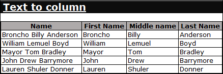
Q10. How we can split a column into 2 or more columns?
Answer: To split the column into 2 or more columns, we use Text to column option.
Example: We have data in range E3:E8 and every cell contains three names with the space. We will follow below steps to split a column into 3 columns:-
- Select the range E4:E8
- Press Alt, A, E on the keyboard
- Text to column dialog box will appear
- Step 1 of 3: Select Delimited, Step 2 of 3:- Click on Space, Step 3 of 3:- Select the destination (where we want to split data).


- Click on OK
Q11. What is a Dashboard and what are the important things we should keep in mind while creating a dashboard?
Answer: Dashboard is a technique used to present important information through graphical representation. It is helpful in presenting huge data in a single computer screen so it can be monitored with a glance.
There are few things which should be taken care of, while preparing the dashboards:
1) Minimum distraction
2) Simple, easy to communicate
3) Important data
4) Few Colors
5) Relevant graphs
6) Dashboard should be on single computer screen
Q12. What is the easiest solution to reduce the file size?
Q12. What is the easiest solution to reduce the file size?
Answer: Below are the steps to reduce the file size:
- Find the last cell that contains data in the sheet. Delete all rows and columns after this cell
- To delete the rows, press the key Shift+Space then press Ctrl+Shift+Down on your keyboard
- Rows will get selected till the last row. Press Ctrl+- on the keyboard to delete the blank rows
- To delete the column, Press the key Ctrl+Space then press Ctrl+Shift+Right Arrow key on your keyboard
- Columns will get selected till the last row
- Press Ctrl+- on the keyboard to delete the blank columns
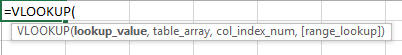
Q13. What is Syntax of Vlookup?
Answer: Vlookup Syntax: =VLOOKUP(lookup_value,table_array,col_index_num,[range_lookup])
Q14. How to select all the objects in the sheet?
Answer: To select the object, we use Go to Special option.
Follow the below steps to select the objects:
- Press the shortcut key F5 to open the Go to Special dialog box
- Click on Special > Click on object > Click on OK
- All objects will get selected

Q15. What is IF function in Microsoft Excel?
Answer: ‘If function’ is one of the logical functions in Excel. We use this function to check the logical condition and specify the value whether it’s true or false. ‘If function’ has three arguments but only first argument is mandatory and other two are optional.

Q16. What is the use of Name box?
Answer: Name Box is located in the left most corner of the Excel sheet. Usually, we use Name box to check the cell reference to the active cell but it has several other uses too.
For Example: We can define the name of the range through Name box. Below are the steps to understand this statement:
- Select the range
- Edit in the Name box
- Type Weeks > Press Enter

Q17. What is the use of Vlookup and how do we use it?
Answer: Vlookup is used to find the data in the large spreadsheet by lookup value in another worksheet. To use the Vlookup function, we should have common values in both data. For example, we want to search the phone number of a person. So, in order to find out the phone number, we will need the concerned person’s name.
How do we use it?
We have 2 set of HR data in Excel. In the second data, we want to update joining date of every employee from the first data. To use the Vlookup function, data must have the common value.

Follow below steps:-
- Enter the formula in cell G3
- =VLOOKUP(F3,$A$3:$D$13,2,0)
- Press enter and copy the same formula in the range F4:F13
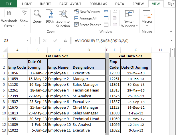
Formula Explanation: =VLOOKUP(F3,$A$3:$D$13,2,0)
- In this formula, F3 is the cell of common value or lookup value
- Then we have selected the range $A$3:$D$13 to the 1st data
- 2: we have defined to pick the value from the 2nd column
- 0: we have defined for the exact match
Q18. How can we view the values in the right most column in Excel?
Answer: We can view the value from the right most column through Index and Match function.
Example: We have 2 HR data in Excel. In the second data, we want to update joining date of every employee, from the first data. To use the Vlookup function, data must have the common value.

Follow below steps:-
- Enter the formula in cell G3
- =INDEX($A$3:$D$13,MATCH(F3,$B$3:$B$13,0),1)
- Press Enter
- Copy the formula in range G4:G13.

Formula Explanation: =INDEX($A$3:$D$13,MATCH(F3,$B$3:$B$13,0),1)
- In this formula =INDEX($A$3:$D$13 this syntax is used to define the array from which we want to pick the value
- MATCH(F3,$B$3:$B$13,0) this syntax will help to lookup the value
- At last ‘1 define’ is to pick the value as result so 1 implies that we want to pick the value from the 1st column
Q19. How can we merge multiple cells text strings in a cell?
Answer: We can merge multiple cells text string by using the Concatenate function and “&” function.
Example: We have three names: First Name, Middle name, Last name in 3 columns. To merge the names and make it a full name, follow the steps below:

Concatenate Function
- Enter the formula in cell D2
- =CONCATENATE(A2,” “,B2,” “,C2)

“&” use in formula to merge the text:
- Enter the formula in cell E2
- =A2&” “&B2&” “&C2

Q20. What is Sumif function and how to use it?
Answer: We use Sumif function to add the cells specified by a given condition or criterion.
| Syntax | Range | Criteria | Sum_Range |
|---|---|---|---|
| =SUMIF(range, criteria,[sum_range]) | Data range from which we want to retrieve the sum | For which we want to calculate the sum from the data | The range of column from which we want calculate the sum |
How to use it?
We have HR data in which we have salary details of every employee, department wise. Now, we want to retrieve the total salary amount department wise.

Follow these steps:
- Enter the formula in cell I2
- =SUMIF($A$2:$E$17,$H2,$E$2:$E$17) and press Enter
- Copy the same formula in the range

Formula Explanation:
- $A$2:$E$17it is the range of data
- $H2 is the criterion for which formula will calculate the sum
- ,$E$2:$E$17is the sum range in the data
Q21. What is Countif function and how to use it?
Answer: We use Countif function to count the specified cells, with a given condition or criterion.
Example: We have HR data with salary details of every employee, department wise. Now, we want to count number of employees department wise.

- Enter the formula in cell I2
- =COUNTIF($A$2:$A$17,H2)
- Copy the same formula for the all manufacturer
Few more examples:
Q22. What is Nested IF function?
Answer: When we have multiple conditions to meet, we can make use of IF function 7 times, which is called Nested IF function.
Example: In cell A1, there is drop down list of A, B, C & D. If A is selected then cell B1 should return Excellent, on selection of B result should be good, for C result should be Bad and D should be poor.

Q23. What is Pivot table and why we use it?
Answer: Pivot table allows quick summarizing of large data. We can calculate the field and arrange the data in presentable way in just few minutes. Most of the Excel experts believe that Pivot table is the most powerful tool.
Why do we use it?
- Pivot table gives us flexibility and analytical power
- It is a time saver source in Excel
- Listing unique values in any column of a table
- Making a dynamic pivot chart
- Linking data sources outside excel and be able to make pivot reports out of such data
Q24. How to use advanced filter?
Answer: We use Advanced filter to extract the unique list of items or we can extract the specific item from different worksheets. We can say that Advanced filter is an advanced version of Auto filter.
Example: In a range, we have duplicate products and we want to filter only unique list.

Follow below steps:
- Select the data range
- Go to Data tab > Click on Advanced
- Advanced dialog box will open
- Click on copy to another location
- Select the destination

- Click on OK

Q25. How we can change the cell formatting?
Answer: To change the cell formatting “Format cell” option is used.
Example: In cell A1, the value is to be converted into percentage, change the number appearance by following these steps:
- Press Ctrl+1 shortcut key to open Format cells dialog box
- In the number category, click on Percentage option
- Click on OK

Q26. What is conditional formatting and how to use it?
Answer: Conditional formatting is a tool that allows us to highlight the cells or range on the basis of few conditions and that formatting is always based on the values or text which can be automatically changed.
Example: In cell A1, there is a drop down list of A, B, C & D. If A is selected, then cell should be highlighted in green color, If B1 is selected then cell color should be blue, in case of C it should be yellow and if D is selected, then it should be highlighted in red color.

Follow these steps:
- Select the Cell A2
- Go to Home Tab > Conditional Formatting > New Rule > Use a formula to determine which cells to format

- Enter the formula in tab
- Click on Format > Format cells dialog box will appear > Fill tab > Choose color > Click on OK
- Follow the same procedure for the rest of the grades

Q27. How to make drop down list?
Answer: We make the drop down list by using the data validation in Microsoft Excel.
Example: We want to create weekday’s list in a cell.
Follow these steps:
Make the weekday’s list in column A.
Select the cell in which we want to create the drop down list.
- Go to Data tab > Data validation > Data Validation dialog box will open
- In Settings tab > List (Allow) > Source (Select the range A1:A8) > Click on ok
- In Cell C1, drop down list will be created


Q28. How to make dynamic drop down list?
Answer: To add item in the list, always create the dynamic list. This list picks the added value automatically and no editing is required within the list. To create dynamic drop down list, we use offset function along with Countif function.
Steps to create the dynamic list:
- Select the cell C1
- Go to the Data tab>Data Validation > Data Validation dialog box will appear

- In the Settings tab >List (Allow)
- Enter the formula in formula box
- =OFFSET(A:A,1,0,COUNTA(A:A)-1,1)
- Click on OK

Q29. How can we determine the day of the week for a particular date?
Answer: By using the Weekday function, we can return to the day of the week of a particular date.
Example: In cell A1, its today’s date and we want to return the weekday and count from Sunday. Follow these steps:
- Enter the formula in Cell B1
- =WEEKDAY(A1,1) press Enter
- Formula will return 3, it means today is 3rd day of the week

Q30. What is chart and how can we use it?
Answer: Chart is the way to represent the data in graphical visualization. We can present the data in a more informative, easy to understand manner by using the chart. In Excel, we have 10 types of charts.
Example: For representation of sales performance chart, bar chart is suitable.
Say, we have manufacturers’ data with purchase price. We want to see the contribution of every manufacturer; therefore, we will use pie chart.
- Select the data range
- Go to Insert tab > Charts > Select Pie Chart

In the above image, we can see very clearly that which manufacturer has contributed more than others and which manufacturer has contributed the least.
没有评论:
发表评论